
Food data represented as data cards
Hier geht es zur Bestellung der Datenkarten. Hier geht es zur Unterrichtsreihe und here gibt es eine Druckvorlage
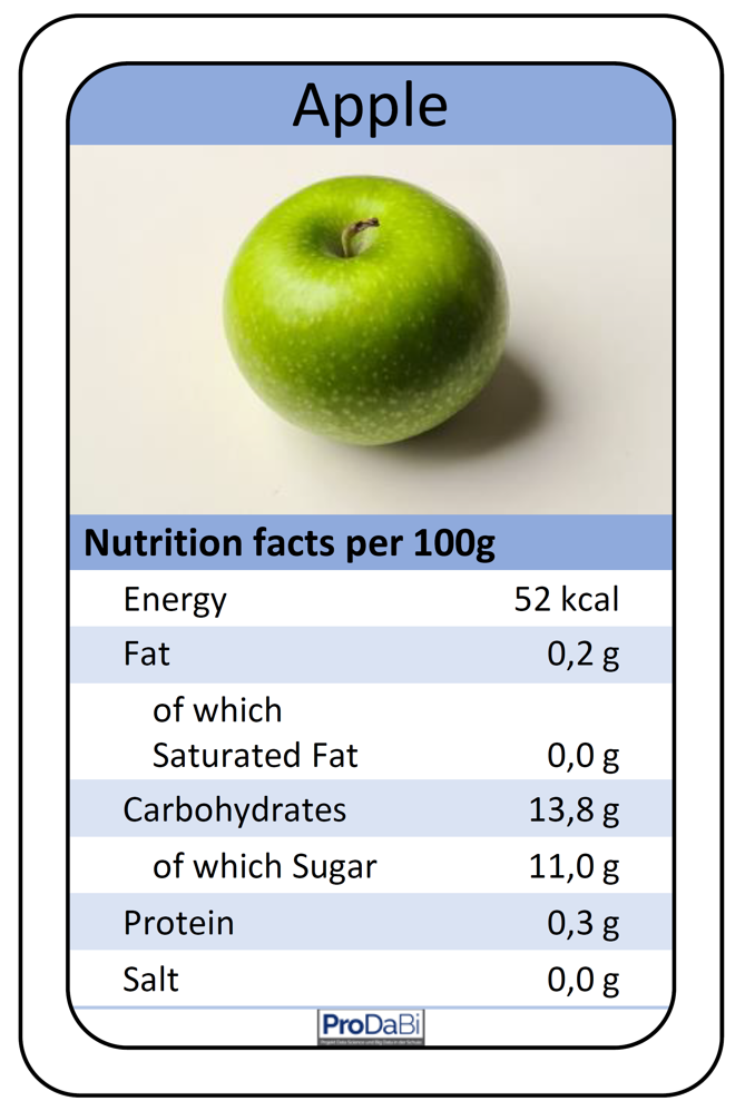
We present here teaching material consisting of 55 data cards, each containing the seven typical nutritional values of a food item, as illustrated for an apple in Fig. 1. Representing food data on data cards as in Fig. 1 and working with such data connects, for example, to the topic of stochastics in the curriculum of North Rhine-Westphalia (NRW) for the lower secondary level (grades 5 and 6). However, from the very beginning, multivariate data—data with several variables—are considered, which has long been emphasized in subject-didactic proposals as an essential component of statistical literacy. Similar connections can also be found in other curricula.
Using the data cards on food items, the teaching is guided by the following key question:
- How can we, using the data cards, construct a recommendation system that classifies a food item, on the basis of its nutritional information, as rather recommendable or rather not recommendable with as few errors as possible?
Such a recommendation system is called a classifier, since individual objects (here: food items) are assigned to a class (“rather recommendable” or “rather not recommendable”) based on their characteristics (nutritional information), i.e. they are classified. The binary variable recommendation is referred to as the target variable, while the numerical nutritional variables are referred to as predictor variables.
Such a classifier is developed on the basis of a set of objects for which both the values of the predictor variables and of the target variable are known. These are the so-called training data. The ultimate goal, however, is that the recommendation also works for new objects. First, the system is tested with test data that were not involved in the training process but for which the values of the target variable are known. This makes it possible to estimate the probability with which the system classifies new objects with an unknown value correctly.
The data example consists of 40 blue cards for creating the recommendation system and 15 yellow cards for testing. Red and green paperclips are used in class to represent the agreed value of the target variable (also called the label).
A decision tree as a classifier
In the following, teachers are introduced to what a decision tree is and how such a tree can be constructed from data using data cards. The didactical implementation in the classroom will be addressed at a later point. A decision tree is a hierarchical system of rules that can be used as a classifier. An example of a decision tree for the previously described context is shown in Fig. 2. This rule system can, for instance, be used to classify the apple from Fig. 1 by traversing the decision tree from top to bottom and, depending on the values of the attributes fat and energy, following the corresponding branches. The first decision node checks the attribute fat. Since the apple contains less than 8 g of fat per 100 g, one takes the left branch and directly arrives at a terminal node (also called a leaf node) of the decision tree. A terminal node is always labeled with a value of the target attribute, which is then assigned to the object being classified. Accordingly, the apple is classified as “rather recommendable.” For a food item with a fat value greater than 8 g, however, one would need to take the right branch and, in a second step, also consider the energy value in order to arrive at a terminal node.
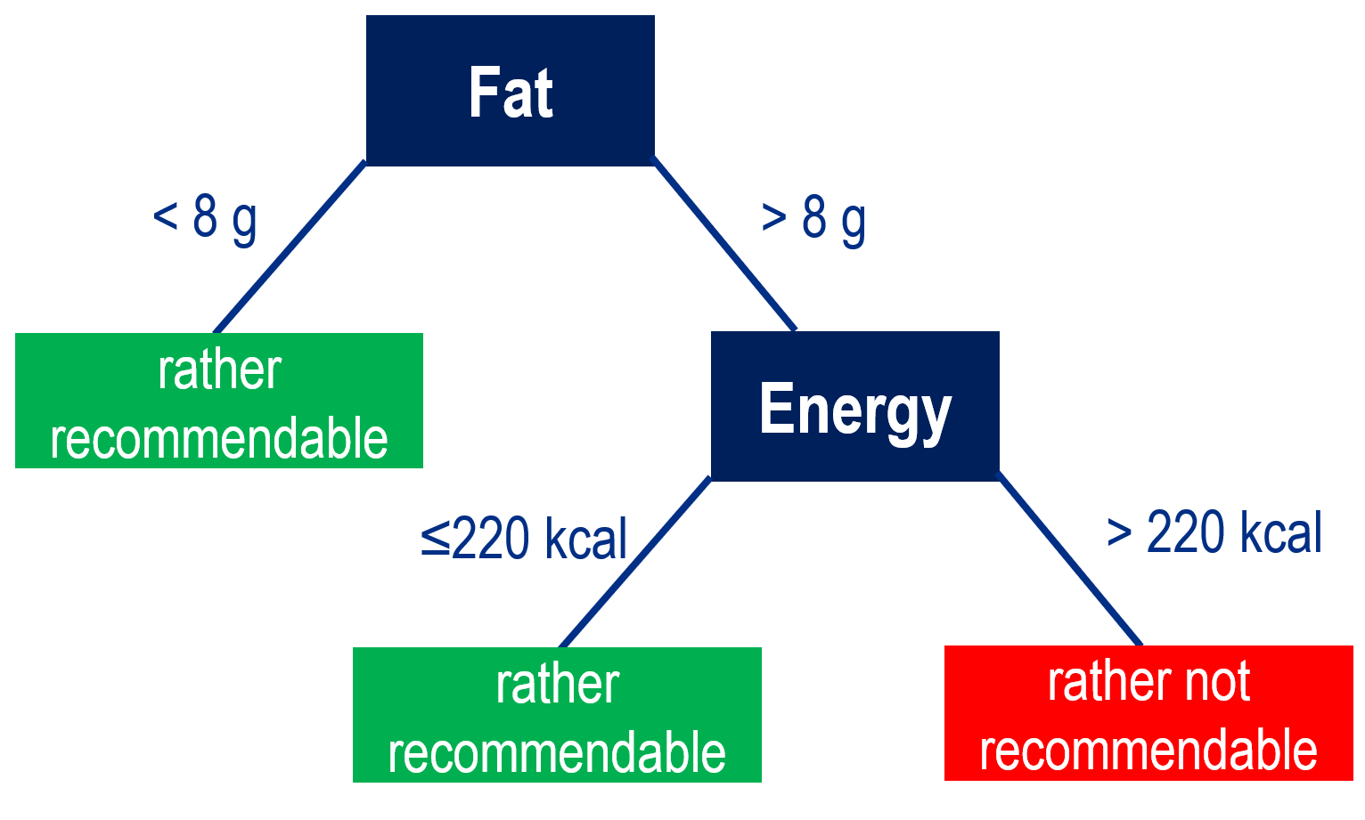
This decision tree is merely an example and does not claim to classify food items in a meaningful way. In principle, such a decision tree can contain any number of levels and predictor variables. The aim of the teaching unit is that students create such a decision tree themselves on the basis of data and understand how computers can be set up to automatically generate decision trees from data (machine learning as part of AI).
Construct a data-based decision tree
A prerequisite for data-based construction of decision trees is the availability of a dataset consisting of a set of example objects for which the values of both the target variable and the predictor variables are known. In the following (Figures 3 and 4), we consider eleven food items as example objects, with their nutritional information specified on each card. These represent the values of the predictor variables such as fat, energy, etc. Furthermore, a green (or red) clip symbolizes whether the food item is classified as rather recommendable (or rather not recommendable), representing the value of the target variable. Based on such a dataset, a decision tree can be built step by step with the aim of classifying the training data with as few errors as possible.
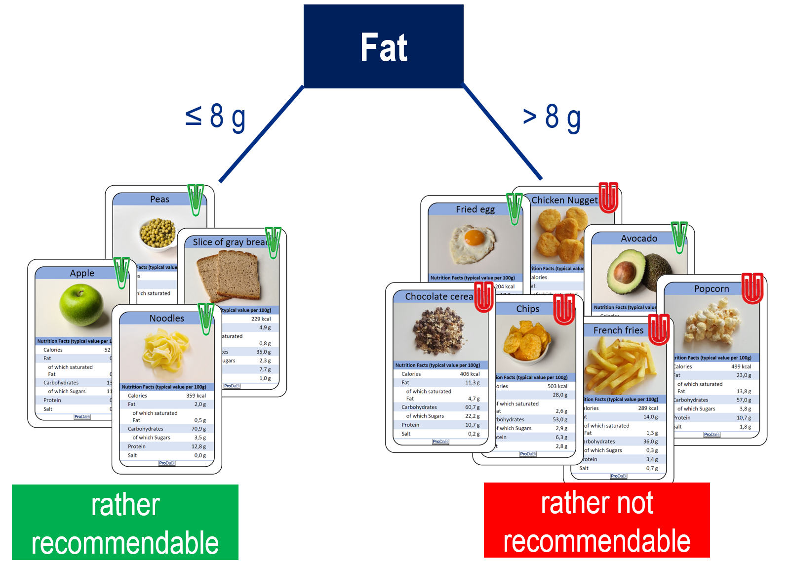
The basis for constructing the decision tree is the so-called data split. That is, using one predictor variable and a threshold value, the dataset is divided into two subsets (Component 1). In Figure 3, we see a data split with the variable fat and the threshold of 8 g, meaning that all food items with more than 8 g of fat are on the right side, and those with up to 8 g of fat are on the left. In each subset, a majority decision regarding the target variable is then made (Component 2). In our example, the left subset contains only rather recommendable food items, while in the right subset the majority of items are rather not recommendable. The resulting decision rule (if ≤ 8 g fat, then rather recommendable; if > 8 g fat, then rather not recommendable) can be evaluated (Component 3) by determining the number of food items misclassified in the dataset (misclassifications). In our example, two food items are misclassified, namely avocado and fried egg on the right-hand side. When constructing a decision tree, data splits are chosen in such a way that these majority decisions produce as few misclassifications as possible. Finally, the resulting one-level decision tree can be represented (Component 4). This can be done verbally or by means of a typical tree diagram. In the representation of the decision tree, the data cards no longer appear. Instead of the cards (cf. Fig. 3), however, the distribution of the target variable in both subsets (4 to 0; 2 to 5) should be noted, so that the number of misclassifications remains transparent.
The one-level decision tree developed so far, which misclassifies two food items, can now be further improved by adding another level. The data cards in the left branch can be set aside, since everything there is already correctly classified. With the cards in the right branch, the procedure is the same as described for the first level. If the predictor variable energy and the threshold of 220 kcal are used for another data split, the resulting decision tree (see Fig. 2) correctly classifies all food items in this dataset.
A central aspect that has not yet been explained is how a variable and a threshold are selected for the first data split and for the subsequent ones in a “favorable” way—i.e., such that as few misclassifications as possible occur. With the data cards, this can be carried out by sorting and systematic trial and error.
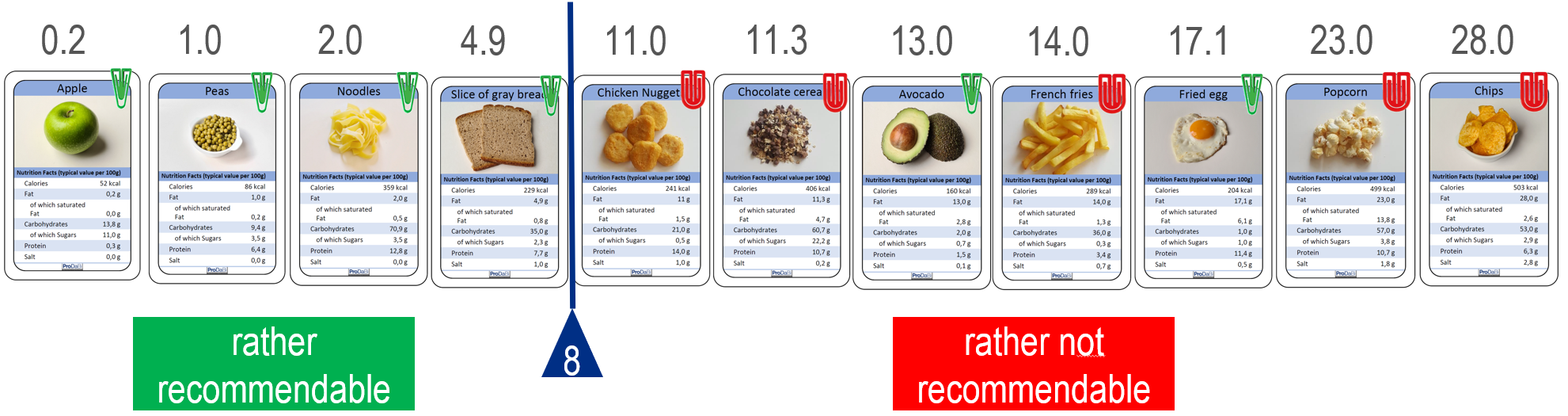
Starting from the sorted data cards, different possible data splits and the resulting number of misclassifications can be compared. For a given dataset, we consider the split to be optimal that produces the smallest number of misclassified objects. In this example, the optimal split is the one visualized in Fig. 4, between the slice of wholemeal bread and the chicken nuggets. This can be verified by systematically examining all possible data splits. To do so, the separating vertical line is shifted step by step into each gap between two cards, and Components 1–3 (as explained earlier) are applied in each case to determine the number of misclassified objects. For example, a split between avocado and French fries results in three misclassified objects and is therefore to be rated as less favorable.
Once an optimal data split has been selected (in our example with two misclassified objects), a threshold can be chosen within the interval between the fat values of the two adjacent cards. In Fig. 4, the value 8 was chosen as the threshold within the interval between 4.9 and 11.0. For all other predictor variables, an optimal split can likewise be determined, after which the predictor variable is selected that yields the smallest possible number of misclassified food items. This means that a so-called greedy strategy is applied: one first searches for the best one-level decision tree, and only then considers the second level and decides whether further splits are required. At each stage, the best variable with its optimal split in the respective subset of the data is selected. It is essentially this systematic method that is implemented in professional decision tree algorithms. These also include suitable stopping criteria. In classroom practice, however, examining all possible splits is very laborious for students, so (initially) somewhat simplified strategies can be applied, which will be explained in the next section. These strategies follow the same approach and can therefore provide a foundation for understanding how a machine proceeds automatically, exhaustively, and systematically.